excel2013突显数字的操作教程
时间:2022-10-26 17:28
有很多小伙伴反映说,自己还不晓得excel2013突显数字的操作,而下文就介绍了excel2013突显数字的操作教程,有需要的伙伴可以参考哦。
excel2013突显数字的操作教程

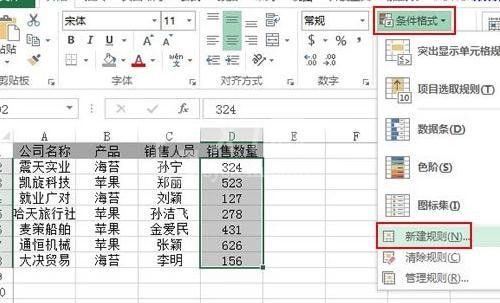
启动excel2013,打开前准备好了的数据表格,选中D2:D8区域,单击菜单栏--开始--条件格式--新建规则。
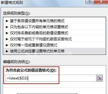
选择最后一个类型,用公式确定要设置格式的单元格,在下方填入公式: =istext($D2) 单击格式按钮,公式的意义稍后介绍。
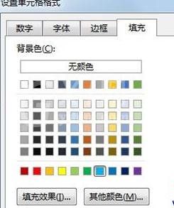
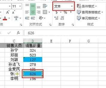
设置单元格的格式,这里以蓝色突出显示。
确定后,会看到有些单元格变为了蓝色,这就是文本格式的数字单元格。
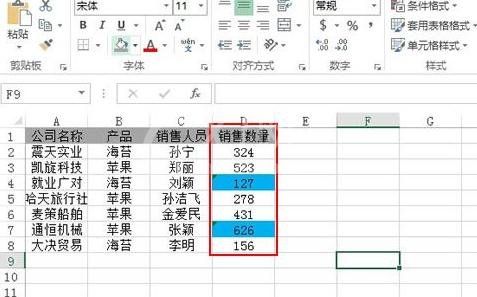
大家能将鼠标单击这些蓝色单元格,看到格式就是文本,证明方法准确无误。
上面就是小编为大家带来的excel2013突显数字的操作方法,一起来学习学习吧。相信是可以帮助到一些新用户的。


热门排行
今日推荐


热门手游
-
商场购物模拟器官方版

版本:v1.0.9
大小:46.11MB
日期:2024-12-16
-
滚动方块大冒险免费版

版本:v1.0.5
大小:26.10MB
日期:2024-12-16
-
恋恋奇缘体验服版

版本:v1.0.0
大小:131.33MB
日期:2024-12-16
-
炉石传说官方正版

版本:v1.0
大小:100.52MB
日期:2024-12-16
-
人群大师免费版

版本:v2.15.0
大小:57.68MB
日期:2024-12-16
-
方鸡跳跑单机版

版本:v1
大小:63.49MB
日期:2024-12-16