excel2007做出帕累托图的操作步骤
时间:2022-10-26 17:40
想必大家都知道excel2007吧,你是否想了解怎样使用excel2007做出帕累托图?下面就是excel2007做出帕累托图的操作步骤,赶紧来看一下吧。
excel2007做出帕累托图的操作步骤

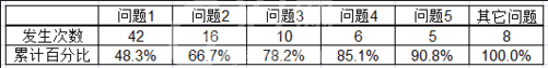
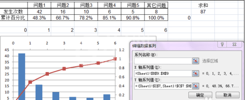
我们先根据你要做的柏拉图的几个要点(反映到图中就是横坐标)列出来,每个要点对应的数量和累计百分比是多少,按照从大到小排列,如果要点很多,只需取前几个要点,如图:假设有10个问题点,我只列出前5项,后5项发生的数量很少这里并作其他问题点
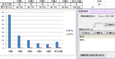
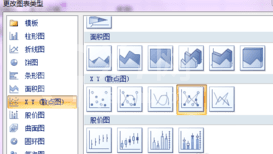
然后我们插入柱形图,选择2个系列,分别对应2个纵坐标轴,这个应该没问题吧
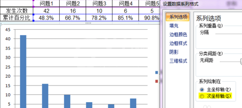
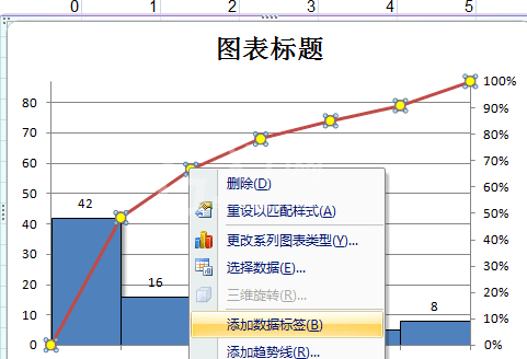
接着我们选择第二个系列,就是红色那个柱状图,右键选择设置数据系列格式,选择次要坐标轴,就是我涂了黄色的那块,然后再选择红色柱状图,右键选择更改系列图标类型,选择XY散点图,如下图
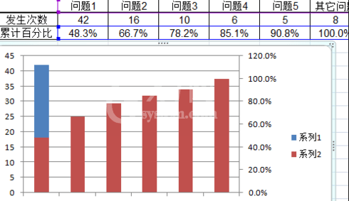
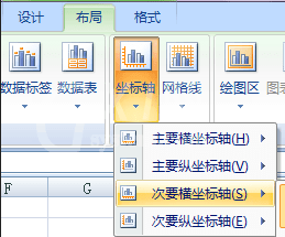
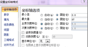
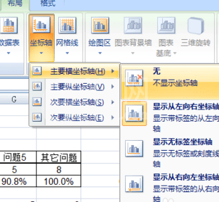
这个时候我们选择图表,在上面菜单栏里选择显示次要横坐标轴,并把坐标轴范围设置为最小值是0,最大值是6,(因为这里我列出了6个问题点);然后再选择红色的折线图,设置X轴和Y轴的数据,注意X周选择0-6,Y周第一个数据选择0,然后按照顺序选择百分比的数据,如图
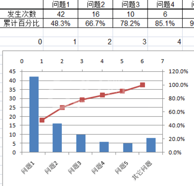
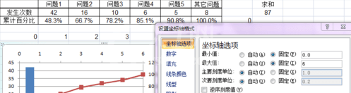
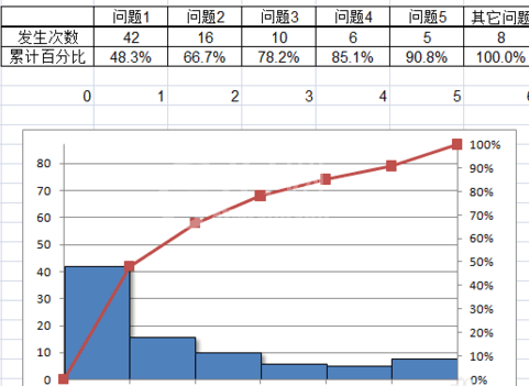
选择哪个折线图,右键选择设置数据系列格式-系列选项-次坐标轴,就变成如下所示:把图例和次要横坐标轴删掉,更改左边和右边的纵坐标轴,左边改为求和的数值87,最小值是0;右边最小值是0,最大值是1,顺便改下数字显示类型为百分比;
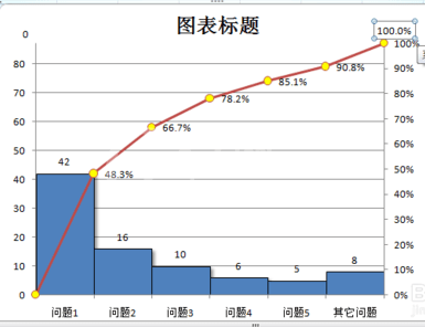
再选择蓝色柱状图,设置数据系列格式,间距调为0,边框黑色,可以设置阴影这样效果要好点;选择红色的折线图,设置数据系列格式,选择数据标记选项,把小圆点调出来,然后把填充色改黄色或其他颜色,这样就基本成型了,
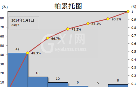
最后我们做一些细节调整,首先把标题提出来;然后右键蓝色柱状图,添加数据标签,然后右键红色折线图,添加数据标签;点中间区域,把主要横网格线去掉(可以选个填充色);再把折现图的数据标签的0和100%这2个标签分别拖到左上角和右上角,用于填写单位,最后再插入一个文本框输入日期和n,就大功告成了。
上文描述的excel2007做出帕累托图的操作步骤,大家是不是都学会了呀!


热门排行
今日推荐


热门手游
-
商场购物模拟器官方版

版本:v1.0.9
大小:46.11MB
日期:2024-12-16
-
滚动方块大冒险免费版

版本:v1.0.5
大小:26.10MB
日期:2024-12-16
-
恋恋奇缘体验服版

版本:v1.0.0
大小:131.33MB
日期:2024-12-16
-
炉石传说官方正版

版本:v1.0
大小:100.52MB
日期:2024-12-16
-
人群大师免费版

版本:v2.15.0
大小:57.68MB
日期:2024-12-16
-
方鸡跳跑单机版

版本:v1
大小:63.49MB
日期:2024-12-16